Many years ago I built a headphone amp based on ESP’s project 113. I always thought it just “sounded good” but never really tested how good it sounded. Now I have an HP 8903A Audio Analyzer and I can be really sure of how good it sounds… by quantifying it!
The 8903A
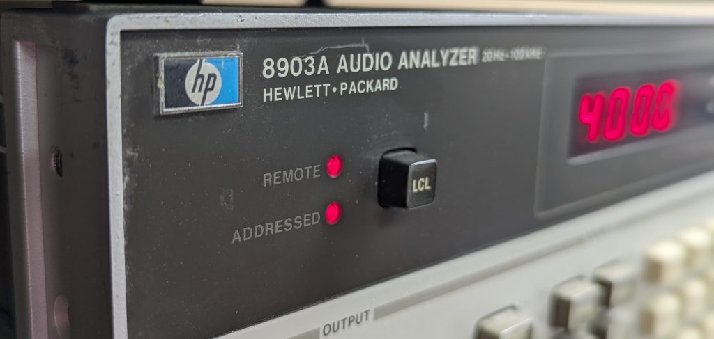
The HP 8903A Audio Analyzer is a precision instrument for testing and analyzing audio equipment and signals. Released by Hewlett-Packard in the mid-1980s, it became a go-to tool in electronics labs and production lines for audio devices. The analyzer combines signal generation and measurement in a single unit, making it super convenient for engineers working on amplifiers, filters, and other audio circuits.
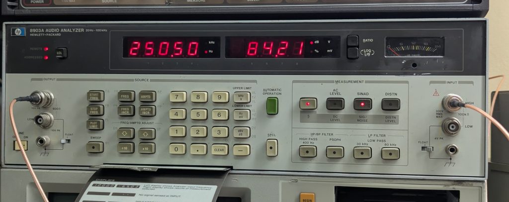
Basically it generates arbitrary tones, from 20Hz to 100KHz in its output port, and then it measures the same tone at the input, after passing through the DUT. It can measure a bunch of parameters like amplitude, distortion, SNR, DC level, SINAD, and it can do some calculations too – to display the outputs in % or dB, or even special functions to calculate power in watts given the output impedance.
The amplifier
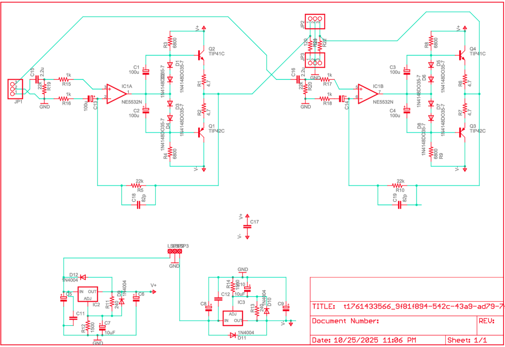
The amp is a “classic” design, based on a stereo opamp, and push-pull outputs with bipolar transistors. The details are at the project’s page: https://sound-au.com/project113.htm and my only modification is that I included the power supply. I used LM317/LM337 to regulate the +/-V rails. Here’s a bad capture of the schematic:
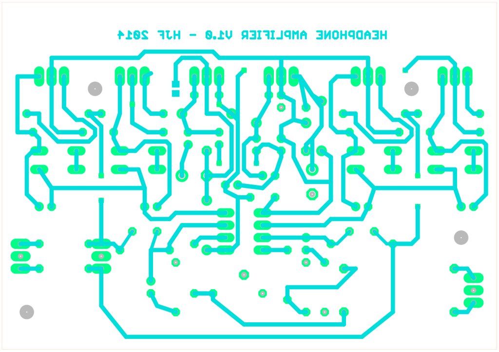
And the PCB I designed:
For the opamp, I used a classic NE5532, an old bipolar opamp specifically designed for audio. It’s still pretty low noise and widely used. For transistors, I used TIP41C/TIP42C for no reason other than I had TIPs handy.
Loading the amp
The first thing I’ll need is a load. A load is just a resistor where I’ll be dumping power. In this case, I used a few resistors in parallel, not because I needed any significant amount of power (this amp, in the tested conditions, outputs a fraction of a watt), but to avoid stray inductance.
Stray inductance in resistors can introduce unwanted phase shifts or impedance variations, especially at high frequencies, which could skew the measurements.
Inductance follows the same rule as resistance when combining it. Resistors in parallel decrease resistance, and inductors in parallel decrease inductance. By placing multiple resistors in parallel I can decrease inductance.
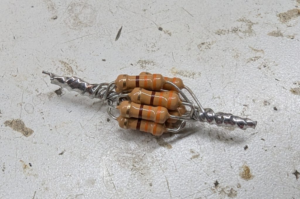
I built two loads for this project. One for around 33 ohms (typical headphones are around 30-40 ohms), and another for 330 ohms (“high impedance” headphones are around 250-300 ohms. Some rare ones even higher). I used ten 330 ohm resistors for the 33 ohm load, and ten 3300 ohm resistors for the 330 ohm load
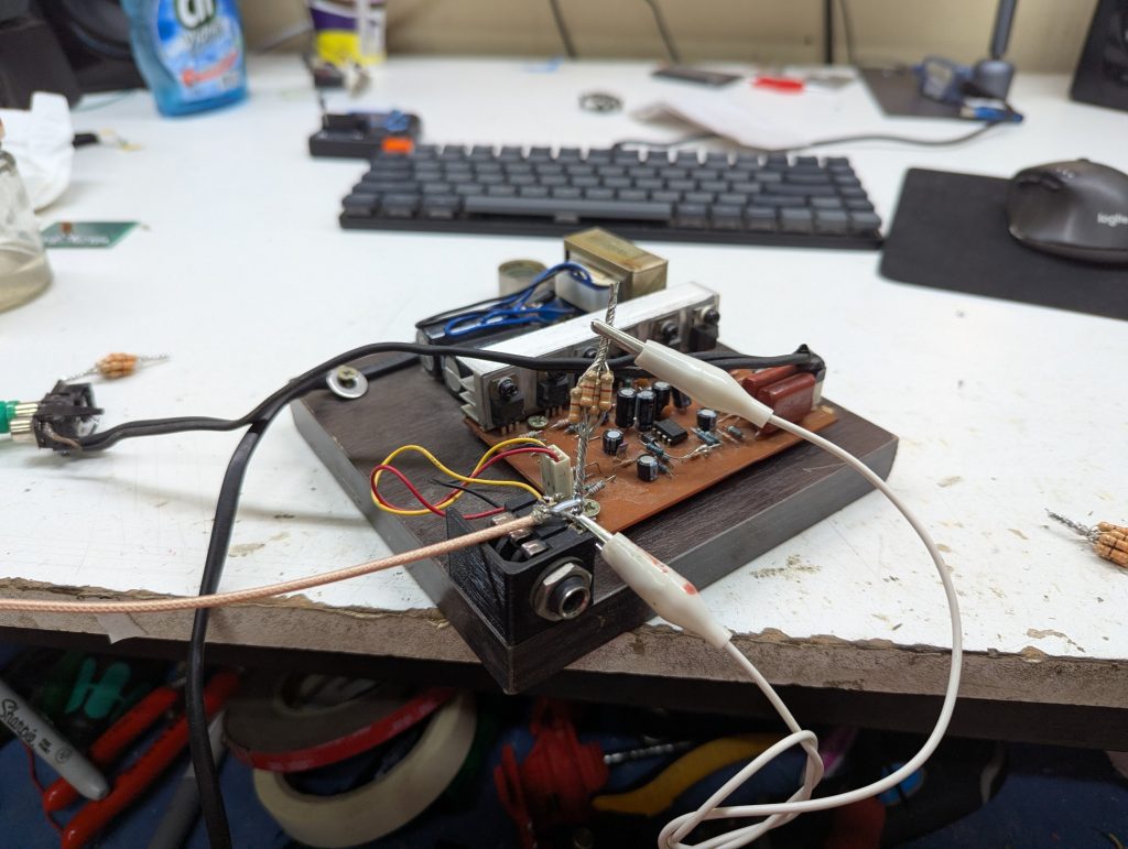
Wiring everything up
Wiring is pretty straightforward. The output (signal generator) of the 8903A is connected to the amp’s input. The input of the amp is connected to the 8903A’s input. In addition, we connect the load between the amp’s output and ground.
Once everything is connected, it’s very simple:
- Press FREQ, enter 20 Hz
- Press AMPLITUDE. Write down the amplitude
- Press DISTORTION. Write down the distortion
- Press S, SNR. Write down the SNR
- Enter the next frequency in the list, and repeat all these steps again
Of course, this is tedious, error prone, and as a hobbyist I don’t have an intern I can task with doing this. The 8903A does support sweeps to automate this a little bit, and it can also output to an XY plotter but of course I don’t own such a device.
So the next best thing is to use GPIB to write a small Python script that will perform these steps thanks to linux-gpib and PyVisa, and write them to a CSV file.
Here is the raw data output for the 33 ohm load.
Frequency(Hz),Amplitude(V),Distortion(%),SNR(dB)
20,1.136,0.0088,80.04
25,1.273,0.0093,81.34
31.5,1.399,0.0082,82.47
40,1.501,0.0074,83.39
50,1.573,0.0058,83.77
63,1.626,0.0068,83.88
80,1.663,0.0068,84.18
100,1.687,0.0066,84.38
125,1.702,0.0068,84.88
160,1.714,0.0073,84.52
200,1.721,0.0075,84.56
250,1.725,0.0068,84.44
315,1.727,0.0071,84.72
400,1.728,0.0069,84.22
500,1.73,0.0075,84.24
630,1.731,0.0071,84.37
800,1.731,0.0069,84.0
1000,1.732,0.0075,84.29
1250,1.733,0.0076,84.03
1600,1.733,0.0086,83.24
2000,1.733,0.0084,83.33
2500,1.732,0.0084,83.0
3150,1.732,0.0082,83.19
4000,1.73,0.0084,83.37
5000,1.729,0.0086,84.03
6300,1.727,0.0085,84.17
8000,1.724,0.0089,83.96
10000,1.719,0.0097,84.25
12500,1.711,0.0105,83.84
16000,1.697,0.0117,83.67
20000,1.679,0.0129,83.67
We can analyze this very easily by pasting it into Excel or Google Sheets, use the Data function to split text into columns, and then just select cells and generate a chart.
But I decided to make it a little more fun and use Python in a Jupyter Notebook to analyze this data.
First some extra calculated columns (gain is calculated based on a 550mV input voltage)
| Frequency(Hz) | Amplitude(V) | Distortion(%) | SNR(dB) | Gain | Gain_dB | Power_mW | Relative_Gain_dB |
|---|---|---|---|---|---|---|---|
| 20.0 | 1.136 | 0.0088 | 80.04 | 2.1 | 6.30 | 39.106 | -3.67 |
| 25.0 | 1.273 | 0.0093 | 81.34 | 2.3 | 7.29 | 49.107 | -2.68 |
| 31.5 | 1.399 | 0.0082 | 82.47 | 2.5 | 8.11 | 59.309 | -1.86 |
| 40.0 | 1.501 | 0.0074 | 83.39 | 2.7 | 8.72 | 68.273 | -1.25 |
| 50.0 | 1.573 | 0.0058 | 83.77 | 2.9 | 9.13 | 74.980 | -0.84 |
| 63.0 | 1.626 | 0.0068 | 83.88 | 3.0 | 9.42 | 80.117 | -0.55 |
| 80.0 | 1.663 | 0.0068 | 84.18 | 3.0 | 9.61 | 83.805 | -0.36 |
| 100.0 | 1.687 | 0.0066 | 84.38 | 3.1 | 9.74 | 86.241 | -0.23 |
| 125.0 | 1.702 | 0.0068 | 84.88 | 3.1 | 9.81 | 87.782 | -0.16 |
| 160.0 | 1.714 | 0.0073 | 84.52 | 3.1 | 9.87 | 89.024 | -0.10 |
| 200.0 | 1.721 | 0.0075 | 84.56 | 3.1 | 9.91 | 89.753 | -0.06 |
| 250.0 | 1.725 | 0.0068 | 84.44 | 3.1 | 9.93 | 90.170 | -0.04 |
| 315.0 | 1.727 | 0.0071 | 84.72 | 3.1 | 9.94 | 90.380 | -0.03 |
| 400.0 | 1.728 | 0.0069 | 84.22 | 3.1 | 9.94 | 90.484 | -0.03 |
| 500.0 | 1.730 | 0.0075 | 84.24 | 3.1 | 9.95 | 90.694 | -0.02 |
| 630.0 | 1.731 | 0.0071 | 84.37 | 3.1 | 9.96 | 90.799 | -0.01 |
| 800.0 | 1.731 | 0.0069 | 84.00 | 3.1 | 9.96 | 90.799 | -0.01 |
| 1000.0 | 1.732 | 0.0075 | 84.29 | 3.1 | 9.96 | 90.904 | -0.01 |
| 1250.0 | 1.733 | 0.0076 | 84.03 | 3.2 | 9.97 | 91.009 | 0.00 |
| 1600.0 | 1.733 | 0.0086 | 83.24 | 3.2 | 9.97 | 91.009 | 0.00 |
| 2000.0 | 1.733 | 0.0084 | 83.33 | 3.2 | 9.97 | 91.009 | 0.00 |
| 2500.0 | 1.732 | 0.0084 | 83.00 | 3.1 | 9.96 | 90.904 | -0.01 |
| 3150.0 | 1.732 | 0.0082 | 83.19 | 3.1 | 9.96 | 90.904 | -0.01 |
| 4000.0 | 1.730 | 0.0084 | 83.37 | 3.1 | 9.95 | 90.694 | -0.02 |
| 5000.0 | 1.729 | 0.0086 | 84.03 | 3.1 | 9.95 | 90.589 | -0.02 |
| 6300.0 | 1.727 | 0.0085 | 84.17 | 3.1 | 9.94 | 90.380 | -0.03 |
| 8000.0 | 1.724 | 0.0089 | 83.96 | 3.1 | 9.92 | 90.066 | -0.05 |
| 10000.0 | 1.719 | 0.0097 | 84.25 | 3.1 | 9.90 | 89.544 | -0.07 |
| 12500.0 | 1.711 | 0.0105 | 83.84 | 3.1 | 9.86 | 88.713 | -0.11 |
| 16000.0 | 1.697 | 0.0117 | 83.67 | 3.1 | 9.79 | 87.267 | -0.18 |
| 20000.0 | 1.679 | 0.0129 | 83.67 | 3.1 | 9.69 | 85.425 | -0.28 |
I did the same for the 330 ohm file, and then got this nice chart:
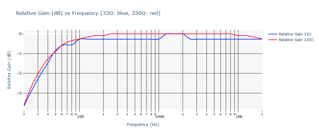
We can see that the response on the low end isn’t super flat. There is a -3dB point at around 25Hz, and it affects both versions. This is more than likely due to the input capacitors not being large enough. I may have to replace the input capacitors but I’m not terribly worried about this, as it’s served me like this for over a decade now.
Let’s now focus on the 1KHz lines of the CSV files which is where specs are usually defined. I had to use an input voltage of 550mVpp in order to test this as the gain is a bit too high for the usual 1Vpp without clipping.
| 33 ohm | 330 ohm | |
| Output Vrms | 1.732 | 5.67 |
| Gain (times) | 3.1 | 10.3 |
| Gain (db) | 9.83 | 20.26 |
| Distortion | 0.0075% | 0.0071% |
| SNR (*) | > 84 dB | > 84 dB |
| Power (mW) | 91 | 97 |
(*): One important thing we need to note here is that the 84dB figure for the SNR isn’t accurate. As it turns out, my little amp is better than the device I’m using to measure it. Let’s look at the specs of the 8903A:
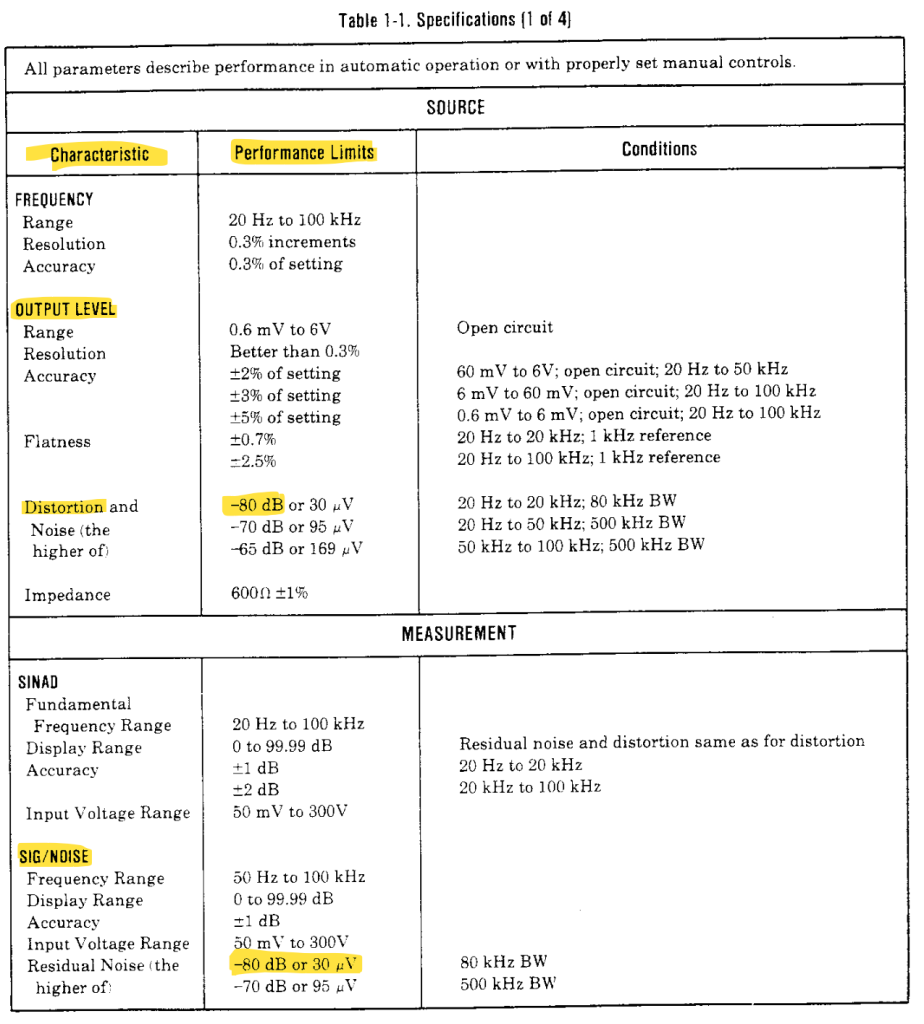
We can see that the residual noise is an absolute minimum of -80dB. Then:
So basically it measures the level of the signal, vs the level of the silence. The 8903A is noisier than this headphone amp. We can confirm this by connecting a straight-thru cable between the 8903A’s input and output connectors and if we assume the cable’s noise to be zero (certainly it will be less noisy than any silicon junction!), we’ll see the same number, around 80-85 dB SNR, meaning the 84 dB SNR is more a limit of the analyzer than of the amp itself.
Putting numbers in context
We can see that sometimes things are good enough. 85dB is already great. Imagine that a quiet room still has around 20dB of noise (less than this and you start hearing your own blood flowing through your veins). 85dB is already excellent, and more than this is superlative. Modern amps boast numbers like 120+ dB which are great in theory (“more is better”), but this is diminishing returns territory. You will not hear this.
The distortion this amp provides is also ridiculously low. 0.0075% is silly. Imagine that most commercial amps will publish power ratings at 1% THD (and subwoofer amp ratings will even be at 10% THD!). Good ones, however, will rate their power at 0.1% THD.
The output power provided is also absurdly high. But this is a good thing: it’s all about the headroom. It’s not about listening loud, but about listening at a comfortable level AND having headroom for sound to go higher when needed.
I’ve tried it with several headphones. Let’s look at the specs of some nice headphones from Sennheiser, the HD660S2, which work very well with this amplifier:
| Total harmonic distortion (THD) | <0.04% (1 kHz, 100 dB) |
| Sound pressure level (SPL) | 104 dB (1 kHz, 1 Vrms) |
This means that at 90mW RMS we’re hitting around 85dB with these headphones. It doesn’t sound like much, but it is. This is more than enough power to saturate the low end (you can hear the driver slapping inside the headphone).
You can, however, get more power out of this thing. The output of the amp is actually limited by a 120 ohm resistor. Reducing this by half will increase the power to 250mW. Removing it completely (I can’t advise this) would theoretically give you around 7 watts at 8 ohms. Meaning this little amp could easily drive some decent desk speakers with enough power to give them some low end!
And yes, I’ve tried measuring directly, bypassing the limiting resistor
The output at 33 ohms was 6.95Vpp. Distortion of 0.075%, SNR >84, and a whooping 1.47 Watts RMS. That’s what I call overkill.
Audiophool-proof performance
There are plenty of headphone amplifiers out there nowadays. Expensive ones (upwards of $200) promise miraculous sonic revelations, but in reality, they offer nothing you could actually hear compared to this little, cheap amp cobbled together from 40-year-old parts that any well-stocked hobby lab would have. Other components in your chain might be quietly sabotaging your sound, and yet this humble amp is already more than enough. Beyond this, all the numbers, dB claims, and “superior fidelity” marketing are just glitter — meaningless specs for the average listener. At this point, you’re already scraping the limits of human hearing, especially if you’re over 30, live in a city, and have ears that have survived decades of traffic, concerts, and headphone marathons.
One reply on “Headphone Amplifier Tested: Why Expensive Gear Sometimes Doesn’t Matter”
This is a very interesting analysis, I ended up purchasing expensive audio gear from a company No denying that their amp is good but but your project shows that it is possible to get identical performance for a fraction of the cost. Thanks for sharing.